Category Archives: Operations Management

Forecasting Attendance at Baseball Games

Here is a pdf of my most recent school project: Predicting Day-to-Day Variability in Baseball Attendance to Support Staffing

It details how I used 30 years of attendance data at MLB games to determine what is important in predicting attendance. A lot of businesses surrounding stadiums rely upon accurate forecasts of attendance in order to staff their business appropriately. If the effect of short-term factors (weather, recent performance) dominate, schedulers would do well to wait until the last minute to put out a staff schedule. However, it seems that long-term factors (date/time of game, opponent, performance in past seasons) dominates the attendance regression, giving schedulers the ability to put out schedules well in advance of gameday. A missing short-term regressor in my paper is pitching matchup. If star starting pitchers really bring more fans to the game, that might increase the importance of the short-term factors.

Theory Thursday- Conditional Probability

Now that we know the Three Axioms of Probability, we can understand conditional probability.

First, let’s think about a normal (unconditioned) event. What is the probability of rolling an 8 with 2 normal dice (equally likely outcomes from 1 to 6)? Well, we can roll a 2-6, 3-5, 4-4, 5-3, and 6-2 with the two dice to get a sum of 8. That’s 5 possible outcomes that sum to 8. There are 36 possible outcomes, so the probability is 5/36.

The conditional probability of an event is the probability that the event happens, given that another event has happened or will happen. So, for example, what is the probability that I roll an 8 with 2 dice, given that the first die is a 2? Well, I would need the second die to be a 6 for them to add to 8, and there are 6 options for the second die. So I have a conditional probability of 1/6 of rolling an 8, given that the first die was a 2. The conditional probability of rolling an 8 given the first die is a 2 (1/6) is higher than the unconditioned probability of rolling an 8 with 2 dice (5/36).

What is the conditional probability of rolling an 8 with 2 dice, given that the first die is a 1? Well, we would need the second die to be 7. But the die only has options from 1 to 6. So we cannot roll an 8 with 2 dice if one of the dies is a 1. The conditional probability is 0.

We have an easy way to calculate the probability of a conditional event happening. Let E be the event we want to happen, conditional on the event F happening. Let P(E|F) be the conditional probability of E given F. Then P(E|F)=\frac{P(EF)}{P(F)}, where P(EF) is the probability of both E and F happening.

In our example with the dice, E=roll an 8 with 2 dice and F=roll a 2 with the first die. There is one way to roll an 8 with two dice and roll a 2 with the first die: 2-6. There are 36 possible outcomes, so P(EF)=1/36. P(F)=1/6 because there is a 1 in 6 chance of rolling a 2 with the first die. P(E|F)=\frac{1/36}{1/6}=1/6, as we found above.

Theory Tuesday- 3 Axioms of Probability

Everyone has an intuitive concept of chance/probability. When we say that there is a certain probability of an event happening, what do we mean?

First, you need to understand the concept of an “event”. An event is one possible outcome of some probabilistic scenario. Say you are flipping a coin. The two possible events are “heads” and “tails” (though I guess you could argue that there is a third event: “coin lands on its edge”). As you will see in Axiom #3, since a coin cannot land on both “heads” and “tails, “heads” and “tails” are mutually exclusive.

coin-flip-bbdc392d

There are three axioms upon which probability theory is built:
1. Let P(E) be the probability of an event. Then 0 \leq P(E) \leq 1. The probability of any event is between 0 and 1.
2. Let S be the set of all possible events. Anything that could possibly happen is contained in S. P(S) = 1. The probability of some event happening is 1.
3. Let E_1, E_2, …, E_n be a sequence of mutually exclusive events. Two events are mutually exclusive if only one of the two can happen at any time. P(\cup_{i=1}^n E_i)=\sum_{i=1}^n P(E_i). This says that you can add the probabilities of two or more mutually exclusive events together to get the probability of any one of them happening.

With these three axiomatic building blocks, all of probability theory can be built.

Book Review- Mathletics

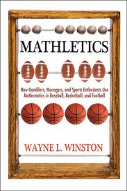
Mathletics: How Gamblers, Managers, and Sports Enthusiasts Use Mathematics in Baseball, Basketball, and Football
By Wayne Winston, 2012 edition

mathletics

I met Wayne in October 2013. I knew that I had one of his books about operations research, but didn’t know much about him. After meeting with him and doing a little research on my own, I’ve learned that he has written an infinite number of books and that he is very skilled at Excel and at sports analytics (among many other things). This book gives intuitive ways to model sports questions and perform analysis with Excel. Example questions include:
-Should we go for the one-point or two-point conversion?
-Should we foul at the end of a basketball game in which we are up 3 points?
-How do different baseball ballparks affect game outcomes?

I’m not a huge fan of analysis in Excel, but Wayne is a wizard at it. I prefer to do a lot of customized number crunching via a programming language (Python/R/Matlab), as opposed to massaging Excel to get what I want. However, this book gave me a lot of ideas for future analysis. It’s kind of a tough read, in that it has 51 chapters over 340 pages and starts/stops thoughts pretty quickly. There are also a lot of editing mistakes in my version, which can sometimes be confusing if you’re not paying attention. I read Mathletics over the span of about 8 months, starting and stopping frequently. I’m glad I finished it, though, because some of the best chapters are in the last part of the book.

Theory Tuesday- Newsvendor Setup

Let’s say you’re a newsvendor. You sell news(papers) or some other perishable good. You used to be a “newsboy”, but now we’re gender-sensitive, so you’re a “newsvendor”.

carrier2

In the morning, you buy/build/accumulate an amount of product. You want to sell all of your product (newspapers/pastries/flowers/perishable widgets) by the end of the day. All the left-over product goes to waste. But you don’t wan to run out of product too early, or you’ll miss out on potential customers who want to buy your product later in the day.

The balancing act between having too much product and having too little product makes this setup ideal for an optimization. Operations research can tell you how much of your product to have in inventory at the beginning of the day to maximize your profit.

Let’s say your product costs $c to buy/build/accumulate. And it sells for price $p to customers. Then your profit, if you stock q quantity and see demand D is: p*min(q,D)-c*q. You only sell the minimum of q, the inventory you have initially, and D, the number of customers that arrive throughout the day to buy your product.

Every lost-sale (because you were out of inventory) costs you p-c dollars, because that would have been your additional profit if you have another unit of inventory. Every unsold unit of inventory costs you c dollars, the stocking cost.

The optimal order quantity, q, is F^{-1}((p-c)/p), where F() is the cumulative density function for your demand for the day. The easiest way to think about this is that you want to have excess inventory (p-c)/p proportion of the time and “stock out” (sell all of your stock) c/p proportion of the time. So if your product costs you $5 to stock and sells for $8, you want to stock out 5/8 of the time. If you consistently order that amount, you will maximize your profit over time. Sometimes you will stock out and sometimes you will have excess inventory, but you will be maximizing profit. (p-c)/p is called the “critical ratio”.

Think about this the next time you see the vast stock of magazines at a bookstore. Since they never seem to stock out, c/p must be pretty low. i.e. the magazines are pure profit for them.
Book Review- Queueing Methods for Services and Manufacturing

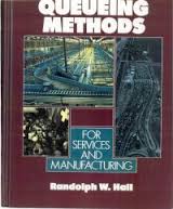
Queueing Methods for Services and Manufacturing
Randolph W. Hall, 1991

queueing

I am reading 4-6 books at any given moment. They range from easy fiction reads to dense technical books, and I read the book that matches my mood and attention span at the time. This summer, I added textbooks to my reading rotation. This is the first textbook I’ve read outside the bounds of a structured class.

This book provides a good overview of options available to diagnose and fix queueing issues. Whether queues are perpetual, predictable, or stochastic, the book discusses them at length. It’s written more for practitioners than academics, in that there are practical diagnostic tools and suggestions for improvement instead of theorems and proofs. There is a good discussion of Little’s Law and steady-state analysis, for those interested in introductory stochastic analysis of queueing systems. I think this is a good book for practitioners and perhaps analytical MBAs, but I don’t know if it dives deep enough into the theoretical backing to be extremely useful for academics. I am glad I read it to get a stronger queueing background, though, and I will reference some of its simpler results and its results on steady-state approximations.

Theory Tuesday- Statistics’ Place in Big Data

Interesting, but long, talk about statistics place in the Big Data world:

I’d suggest watching from about 10 minutes in to about 40 minutes.

“Statistics”, “data mining”, and “bioinformatics” are all on the decline according to Google Trends, while “Big Data” is booming. Many big data people don’t see the need for statisticians because of their seemingly antiquated/belligerent/unhelpful opinions on model validity, result confidence, and experiment design. However, people who ignore statistics are condemned to re-create statistics.

In my experience, the people who don’t see value in statistics are action-oriented and typically mathematically-ignorant. These people want to do something, and they are not especially interested in how accurate their actions are. More responsible big data teams will be built with people with three skill sets: programming, math/statistics, and domain knowledge.

Theory Thursday- Simulation of a Poisson Process

You are using discrete-event simulation to analyze a process or system. Imagine that your arrivals occur according to a Poisson Process. Without using specialized simulation software, this post shows how to code up a Poisson arrival process. Y_n will represent the n’th arrival time.

Stationary arrivals:
If your arrival rate does not vary over time, then your task is easy. You have two main options:
1. Generate exponential random variables X_1, X_2, … , representing interarrival times. Set Y_1 = X_1, Y_2 = Y_1+X_2, Y_3=Y_2+X_3,… Stop generating random variables when Y_m>T for some m, where T is your time interval length that you want to simulate.
2. Generate a Poisson random variable N(T), representing the number of arrivals over a time interval of length T. Then generate N(T) uniform [0,T] random variables, representing arrival times. Sort the arrival times in ascending order to obtain Y_1, Y_2, …

Non-stationary arrivals:
If your arrival rate varies over time, you’ll need an extra step or two of logic to generate your arrival times. Here are two options for simulation:
1. Find the highest arrival rate in your time interval, \lambda_{max}. Generate a stationary Poisson process with rate \lambda_{max} as in option 1 in the stationary arrival section above. For each arrival simulated, generate a uniform[0,1] random variable. If this uniform random variable is less than \lambda(t)/\lambda_{max}, where \lambda(t) is the arrival rate at the generated arrival time, accept the arrival as “real” and keep it. If not, discard the arrival. The “real” arrivals make up an accurate non-stationary Poisson arrival process.
2. Divide the time period [0,T] into small time increments. For each time increment, generate a uniform[0,1] random variable. For each time increment, if the uniform variable is less than or equal to \lambda(t) dt, where dt is the time increment size, then an arrival occurs during that increment. Assign the arrival time to be a random time in the increment. This method is only approximately correct, but it is good enough in most cases and may be faster to simulate in certain cases.

There are other options, but these will get you started in simulating your Poisson processes.

Sacramento Kings Crowdsource Draft Analytics

Painfully interesting mini-movie from Grantland about the Kings’ GM crowdsourcing some of their draft analytics to get fresh ideas.

https://www.youtube.com/watch?v=OuwvsZOvcms

It’s a deep draft. But with my minimal analysis, I don’t seem a huge difference in player potential from the ~4-~20 range. The Kings have the 8 pick, right in the middle of the “really good, but not necessarily great” range. If they can identify some value picks toward the end of the lottery or the late first round, I think it makes sense to move down from the 8 spot if they can get 2 first round picks in return. But I doubt anyone will offer that. Looking forward to seeing what happens in the draft.