When people describe queues in queueing theory, they use a certain notation that at first looks cryptic. For example, a queue that has exponential interarrival times, exponential service times, one server, and room for 10 people in the queue is denoted as an M/M/1/10 queue.

What do the letters in queueing notation mean?

The first letter specifies the probability distribution of interarrival times.
The second letter specifies the probability distribution of service times.
The third letter represents the number of servers working in parallel in the queue.
The fourth letter represents the maximum number of customers in the queue. If omitted, it is assumed to be infinite.

Here are the most common options for the first two letters:
M = exponential (Markovian) distribution
D = deterministic arrival/service times
= gamma distribution with shape parameter n (also called an Erlangian distribution)
G = general distribution (most everything else)

Assumption: You can generate X, a random number from a Uniform[0,1] Distribution. There are many ways to do that.

The objective is to turn X, which is uniformly distributed between 0 and 1, into Y, which is a random number from a probability distribution of your choosing. Examples of probability distributions are the Normal Distribution, Exponential Distribution, and Beta Distributions.

Key insight: All probability values are between 0 and 1. The cumulative distribution function (CDF) for a probability distribution gives the percent of the distribution that is below a value in the distribution. Take X, the number in Uniform[0,1], and transform it into Y, a value in your distribution of interest that has CDF X.

Example: Say you generate X=.766 and want a random number, Y, from the standard normal distribution (mean=0, standard deviation=1). Abbreviate the standard normal distribution as N[0,1]. Let F(x) be the CDF of N[0,1]. To generate Y~N[0,1], we need to find , where is the inverse of the CDF. We can look up in a normal distribution table or by using the function norm.inv(.766,0,1) in Excel. We find that the value of interest is Y=.7257.

For distributions whose CDF is invertible, we can find equations for Y, the random number from the distribution. Take the exponential distribution for example. The CDF of the exponential distribution with mean is . Solve for y. We find . Now, when we generate any X~U[0,1], we can use the equation for to find Y, which is a random number from the exponential distribution.

For distributions whose CDF is not continuous, you will want to find the smallest Y who has a CDF of at least X.

Ralph Keeney wrote an article “Decision Analysis: An Overview” in the journal Operations Research in 1982. It is one of the best expositions on what the field of Decision Science/Analysis actually is.

He first introduces the field as “a formalization of common sense for decision problems which are too complex for informal use of common sense.” The problems that require formal decision analysis methodologies to arrive at a good answer are typically big and messy: many stakeholders, competing objectives, subjective valuations of alternatives, various levels of risk tolerance, and hazy projections. In these situations, four steps are needed:
1. Structure the decision problem
2. Assess possible impacts of each alternative
3. Determine preferences (values) of decision makers
4. Evaluate and compare alternatives

Toward the end of the longish (30+ page) article is this beautiful paragraph:

“Decision analysis embodies a philosophy, some concepts, and an approach to formally and systematically examine a decision problem. It is in no way a substitute for creative, innovative thinking, but rather it promotes and utilizes such efforts to provide important insights into a problem. Philosophically, decision analysis relies on the basis that the desirability of an alternative should depend on two concerns: the likelihoods that the alternative will lead to various consequences and the decision maker’s preferences for those consequences. Decision analysis addresses these concerns separately and provides the logic and techniques for integrating them.”

It is a great article for the layman or young analyst and highly recommended.

Little’s Law or Little’s Formula is a way to relate the average length of a queue and the average waiting time in a queue. It was proved by John Little in 1960 while Little was at the Case Institute of Technology. The paper proving the result is one of the most cited in the field of Operations Research.

Let be the average time a customer spends waiting in a queue. Let be the average length of the queue. Let be the arrival rate to the queue—the average number of people that arrive per unit time. Then the three quantities can be related by the simple formula .

This result holds no matter the arrival process (Poisson, deterministic, etc.), the service process (Poisson, deterministic, etc.), the queueing discipline (first come first served, last in first out, etc.), and the number of servers. It also holds for total time in the system, if you instead use and as the average number of people in the system –combining those in queue and those in service—and the average time in system, respectively. .

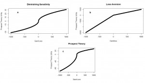
Prospect Theory, created by Kahneman and Tversky, is a way to quantify utility functions for people. In traditional economics, a dollar is a dollar and people are expected to maximize their wealth. In reality, people have biases. The two major biases shown in prospect theory are diminishing sensitivity and loss aversion.

Diminishing sensitivity makes people notice $1 changes in their wealth less the farther that they get from their reference point. $1 means a lot more to someone who is close to breaking even than to someone else who has already made a million dollars.

Loss aversion refers to the fact that people feel losses more strongly than equal sized gains. A loss of $100, relative to your reference point, feels worse than a gain of $100 feels good.

The effects can be seen in the following pictures. (a) isolates diminishing sensitivity and (b) isolates loss aversion. Their combined effects are shown in (c).